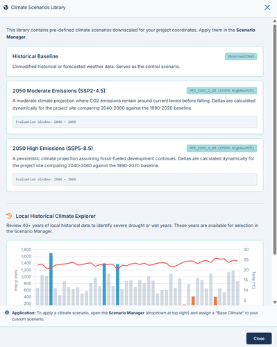
Climate Scenarios
The IAMDD platform allows you to stress-test your hydraulic network and agricultural water demand models against varying meteorological conditions using dynamic Climate Scenarios. Rather than relying on generic regional data, the platform fetches highly localized weather data based on the specific geospatial coordinates of your project using the Open-Meteo API suite.
You can configure scenarios to simulate either observed historical extremes or predicted future climate change projections, allowing you to assess infrastructure resilience and water availability under non-standard conditions.
Local Historical Climate Explorer
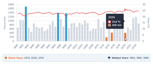
To help identify the most relevant years for stress testing, the Scenario Library includes the Local Historical Climate Explorer.
When opened, this tool queries over 40 years of local historical data from the ERA5 Reanalysis dataset. It analyzes the annual precipitation totals and average maximum temperatures for your specific project location and automatically ranks the data to identify the historically Driest and Wettest years.
This allows you to quickly select bounding conditions for your models without needing to consult external climatology reports.
How Climate Data is Applied to the Simulation
The underlying logic for how weather data is integrated into the hydraulic simulation differs depending on whether you are running a historical year or a future climate projection.
1. Historical Scenarios (ERA5 Reanalysis)
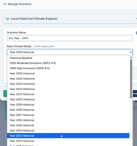
When a specific historical year (e.g., 1983 or 2013) is selected, the simulation engine bypasses the standard baseline weather forecast. Instead, it downloads the exact daily and hourly weather profiles (Precipitation, Maximum/Minimum Temperature, Reference ET, and Wind Speed) that occurred at your project site during that specific year.
The Logic: Because your simulation may be set to run for current or future dates (e.g., April 1 to October 31 of the current calendar year), the engine mathematically proxies the historical data onto your simulation timeline. For example, the weather that occurred on May 15th, 1983, will be applied to May 15th of your simulation window. This ensures that the exact storm events, dry spells, and temperature fluctuations of the extreme year drive the soil-water balance and crop demand models precisely as they occurred historically.
2. Climate Change Projections (CMIP6 HighResMIP)
When a future projection is selected (such as the SSP2-4.5 moderate emissions or SSP5-8.5 high emissions scenarios for 2050), the engine utilizes a perturbation (or "Delta Multiplier") approach.
The Logic: The system first establishes your baseline weather profile (a combination of recent historical data and the 16-day forecast). It then queries the CMIP6 climate models for your coordinates to compare the 1990–2020 baseline averages against the predicted 2040–2060 averages.
From this comparison, the system calculates precise deltas for your site (e.g., Temperature +2.1°C, Precipitation × 0.85, ET0 × 1.05). These multipliers are applied to the baseline daily and hourly weather arrays before the simulation begins. This preserves the natural frequency and timing of local storm events while adjusting their intensity and the background temperature to match the projected future climate.
Example Application: Sizing Infrastructure for Drought Resilience
To understand how this impacts model results, consider a hydrologist designing a municipal and agricultural supply network in the Central Valley of California.
1. Baseline Simulation: The user runs a baseline simulation for the summer irrigation season. The baseline weather provides standard precipitation and temperature inputs. The resulting soil-water balance dictates a certain frequency of irrigation events, resulting in a peak system demand of 2,500 GPM.
2. Identifying an Extreme: The user opens the Local Historical Climate Explorer and identifies 2013 as the driest year on record for the project site.
3. Scenario Configuration: The user creates a new scenario named "2013 Drought Stress" and assigns the Base Climate Model to "Year 2013 Historical".
4. Simulation & Comparison: When the simulation is executed, the engine applies the exact 2013 weather data. Because precipitation is significantly lower and temperatures are higher, the Reference ET increases. The agricultural nodes in the network deplete their soil moisture capacity more rapidly, triggering irrigation events more frequently and for longer durations.
By viewing the Scenario Comparison Chart, the user can overlay the Baseline and 2013 scenarios.
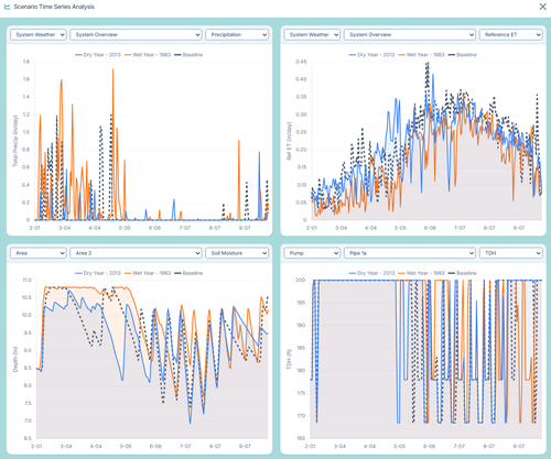
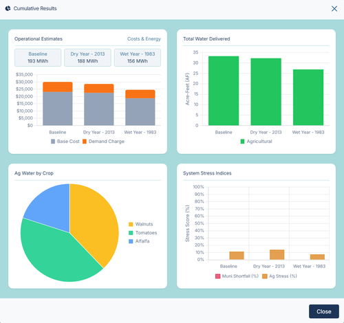
Conclusion: The user visualizes that while the Baseline peak demand was 2,500 GPM, the 2013 historical drought scenario forces the system to sustain 3,200 GPM to prevent crop wilting. This actionable data allows the practitioner to accurately size the pump station and evaluate water right allocations for extreme, rather than average, conditions.