Pressure Boundary Node
The Pressure Boundary is one of the most fundamental hydraulic components in your digital twin. It establishes the hydraulic grade line (HGL) at a specific point in the network, acting as an infinite source or an infinite sink of water.

If you are coming from an EPANET background, the Pressure Boundary is entirely synonymous with the Reservoir node.
Functionality
By definition, a Pressure Boundary maintains a constant hydraulic head regardless of the volume of flow entering or leaving the node.
In both steady-state (EPS) and transient (MOC) simulations, these nodes are crucial for establishing boundary conditions. Common real-world equivalents include: - A large lake, river, or groundwater aquifer providing water to a pump station. - A connection point to a much larger, stable municipal transmission main. - A discharge point open to the atmosphere.
Because it represents an infinite source, the Pressure Boundary itself does not have a finite volume or dynamic water level like a Tank does.
UI Workflow and Configuration
To add a Pressure Boundary to your model, click the Pressure Boundary icon in the Component Toolbar (it resembles a trapezoidal basin) and then drag it onto the canvas to place it.

Once placed, you can configure its boundary conditions by right-clicking the node and selecting Properties.
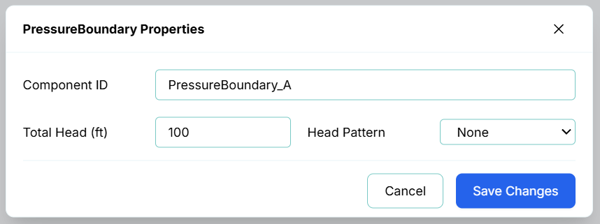
The Properties dialog provides the following configuration fields:
- Component ID: The unique identifier for this node (e.g.,
PressureBoundary_A). - Total Head: The baseline hydraulic grade line (elevation + pressure head) of the water source, measured in your system's length units (e.g., feet or meters).
- Head Pattern: By default, the Total Head remains perfectly constant throughout the simulation. However, you can assign a time-varying pattern to the boundary to simulate fluctuations (such as tidal changes, seasonal aquifer drawdown, or daily pressure swings in a municipal feed).
To assign a pattern, click the Head Pattern dropdown. It will list all the time patterns you have configured in your project (such as Irrigation Demand or Pressure Zone 1).
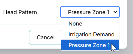
Once you select a pattern (such as Pressure Zone 1), the system will apply a time-varying multiplier to your base Total Head. For example, if you configure the Pressure Zone 1 pattern in the Pattern Modal to dip to 0.8 during peak daytime hours and rise to 1.1 at night, your Pressure Boundary will automatically simulate these real-world diurnal pressure swings throughout the simulation.

Once you have configured the total head and any optional patterns, click Save Changes to commit the boundary condition to the digital twin physics engine.