Hydraulic Components (Nodes & Links)

Source Node

The Source Node represents a point where water enters the network, functioning as either a head-driven hydraulic source or a flow-driven exogenous inflow. It seamlessly consolidates both fixed-head reservoir boundaries and defined-rate flow injection into a single versatile component.

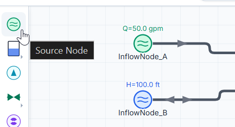
Depending on your modeling goals, the Source Node can be switched between two distinct operating modes:

Reservoir (Fixed Head / Water Elevation): A hydraulically driven boundary that maintains a fixed total head (water surface elevation). Flow is governed dynamically by downstream network resistance and can even reverse into the node if system pressures rise.
Defined Inflow Rate (Flow Injection): A flow-driven exogenous supply that injects a predetermined volumetric flow rate ($Q$) directly into the system, regardless of network pressure.

Operating Modes & Hydraulic Behavior

1. Reservoir Mode (Hydraulically Driven)

In Reservoir Mode (synonymous with an EPANET Reservoir), the node establishes the Hydraulic Grade Line (HGL) at a fixed total head.

How it Works: The node acts as an infinite water source (or sink). The rate of water entering the pipeline is not fixed; instead, it is determined dynamically by the hydraulic gradient, pipe headloss, and pump/valve operations downstream.
Bi-directional Flow: While placed as a source, water can naturally reverse and flow into the reservoir if network pressures exceed the node's total head (for example, during a pump shut-off surge or high downstream storage).
Common Real-World Equivalents:
A large lake, river, or ocean intake.
A connection to a large, high-capacity municipal supply main with known pressure.
An open atmospheric forebay or large clearwell.

[!NOTE] In Reservoir Mode, the node does not have a finite volume or dynamic water level geometry like a Storage Tank. It represents an infinite boundary whose head remains constant unless modulated by a Head Pattern.

2. Defined Inflow Mode (Exogenous Flow Injection)

In Defined Inflow Mode (modeled from an EPANET perspective as a Junction with negative demand), the node forces a specified volumetric flow rate into the system.

How it Works: The inflow rate is treated as an exogenous input. The specified volume of water enters the network every second regardless of the pressure head at the connection point. Unlike a Pressure Boundary (which maintains constant pressure regardless of flow), an Inflow Node delivers constant flow regardless of the resulting system pressure.
Interactive Canvas Sliders: When placed in Defined Inflow Mode, a live slider appears on hover in the modeling canvas, allowing you to manually dial the inflow rate up or down during interactive simulation runs.
Common Real-World Equivalents:
A deep well pump discharging a constant or scheduled flow directly into a manifold.
A metered tributary, river diversion, or upstream watershed inflow.
An unmodeled upstream process plant or booster station delivering a scheduled flow sequence into a municipal grid.
Steady industrial return flows or constant-discharge treatment effluent.

[!TIP] Use Defined Inflow Mode when you know the exact flow rate entering the system (e.g., from flow meter records or pump discharge specifications) rather than the supply pressure.

UI Workflow and Configuration

To add a Source Node to your model: 1. Locate the Source Node icon in the left toolbar. 2. Drag and drop the icon onto the canvas. 3. Right-click the node and select Properties (or double-click) to open the configuration dialog.

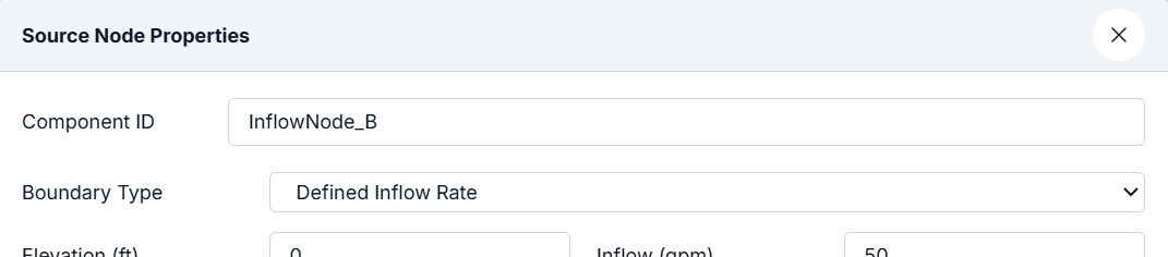
Configuration Fields

Source Mode Selection

At the top of the Properties dialog, select your desired Source Mode: - Defined Inflow Rate (Flow Injection) - Reservoir (Fixed Head / Water Elevation)

Fields in Reservoir Mode

Field	Description
Component ID	Unique identifier for the node (e.g., `Source_1`, `Lake_Intake`).
Total Head	The total baseline hydraulic grade line (elevation + pressure head), measured in feet or meters.
Head Pattern	Optional diurnal or seasonal multiplier pattern applied to Total Head (e.g., simulating tidal shifts, seasonal drawdown, or diurnal grid pressure swings).
Water Quality	Baseline chemical concentration (e.g., Chlorine mg/L), source water age (hours), or constituent percentage for tracking water propagation through the network.

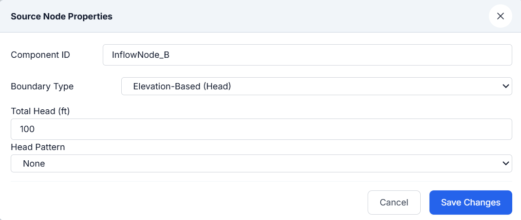
Fields in Defined Inflow Mode

Field	Description
Component ID	Unique identifier for the node (e.g., `Well_A`, `InflowNode_1`).
Elevation	Physical ground elevation of the injection point (length units). This is critical for accurate pressure and HGL calculations.
Inflow	Base volumetric flow rate injected into the network (e.g., gpm, L/s, MGD).
Min / Max Inflow	Lower and upper bounds for live canvas interactive sliders and batch optimization parameter ranges.
Min Pressure	Operational pressure threshold. If system pressure drops below this limit during a simulation, a low-pressure warning triggers in the Telemetry Panel.
Pattern	Multiplier curve that varies the inflow rate over 24-hour diurnal or extended period cycles.
Enable Random Flow	Adds stochastic Autoregressive (AR1) noise to simulate real-world turbulent, un-metered flow variability.
Water Quality Dosage	Chemical dosage (mg/L) injected proportionally with the entering stream for water quality transport tracking.

Flow Rate Patterns (Diurnal Schedules)

In reality, supply and well pumping rates are rarely constant. To accurately model an Extended Period Simulation (EPS) run across multiple days, you can assign a Pattern to the Base Inflow.

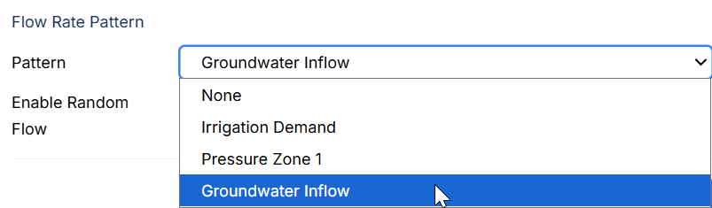
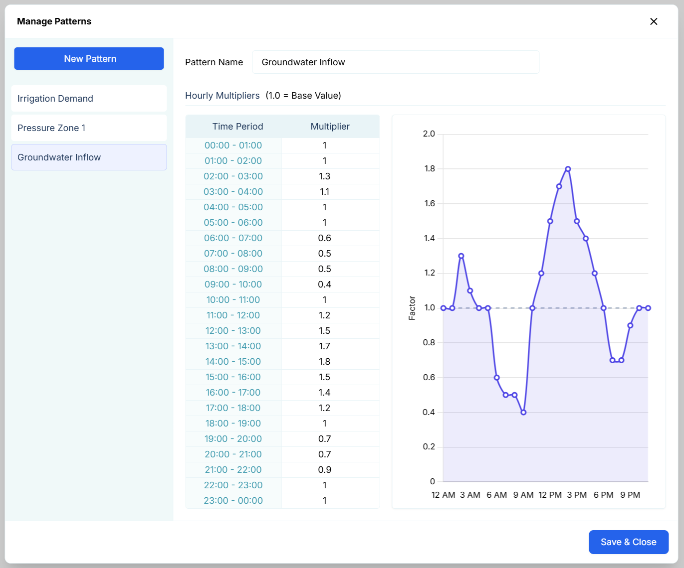
Selecting a pattern (such as Groundwater Inflow) applies a time-varying multiplier to the base Inflow value over the course of the simulation.

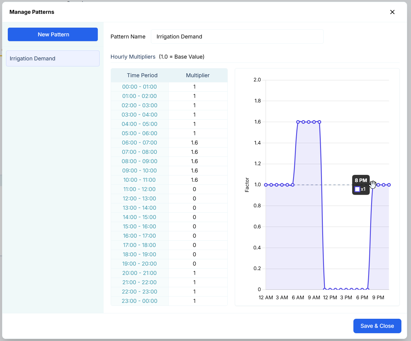
For instance, the Groundwater Inflow schedule shown above models a well pump that runs at 100% capacity (a multiplier of 1.0) during off-peak nighttime hours, and completely shuts off (a multiplier of 0.0) during peak daytime electricity tariff hours to save power. By assigning this pattern, your Source Node automatically adheres to the daily pumping schedule without manual intervention.

To create or edit patterns, open the Manage Patterns dialog from the main toolbar. Patterns can be adjusted numerically or shaped visually by clicking and dragging points on the interactive curve!

Stochastic Inflow (Random Flow)

For advanced modeling, perfectly smooth supply curves do not capture real-world operational turbulence. R-THYM can simulate realistic noise using the Enable Random Flow toggle.

When enabled, the physics engine generates a continuous stochastic noise layer and overlays it onto the base inflow and pattern. You control the behavior with two parameters:

Autocorrelation (0–1): Controls the persistence or "memory" of the random walk:
A value near 0.0 produces high-frequency, choppy white noise.
A value near 0.8 to 0.9 produces a smooth, wandering random walk that closely mimics natural watershed and turbulent pump variations.
Std Dev (Flow Units): The Standard Deviation sets the amplitude or spread of the random fluctuations (e.g., a standard deviation of 10 gpm means inflow will typically vary within $\pm 10$ gpm of the target baseline).

Live Canvas Interaction & Telemetry

Interactive Canvas Slider

During live simulations, hovering over a Source Node configured in Defined Inflow Mode reveals an on-canvas slider. Dragging this slider interactively dials the inflow rate up or down in real time, allowing you to stress-test downstream system response immediately.

Telemetry Panel Monitoring

Clicking any Source Node during a simulation opens its live metrics in the right-hand Telemetry Panel: - Instantaneous Flow & Pressure: Displays the live injection rate (or reservoir withdrawal rate), delivery pressure head, and cumulative volume supplied to the system. - Time-Series Charts: Dynamically plots inflow, pressure, and stochastic fluctuations over the duration of the run. - Low Pressure Alerts: If the pressure at the node falls below the configured Min Pressure threshold, an alert badge is raised to flag supply degradation or potential cavitation conditions.

Solver Mapping & EPANET Export

When your network is solved or exported, the Source Node is translated according to its active mode:

Mode	Steady-State / EPS (EPANET)	Transient Engine (MOC)
Reservoir Mode	Exported to `[RESERVOIRS]` with fixed total head $H$.	Modeled as a constant-head boundary providing full wave reflection ($H = H_{res}$).
Defined Inflow Mode	Exported to `[JUNCTIONS]` with negative base demand ($-Q$).	Modeled as an internal junction with prescribed exogenous flow injection.