Creating and Viewing Charts
In R-THYM, real-time visualization is the core bridge between mathematical hydraulic solving and engineering decision-making. Whether you are running an Extended Period Simulation (EPS) to optimize 24-hour pump energy dispatch or executing a Method of Characteristics (MOC) dynamic transient analysis to protect a pipeline against water hammer, R-THYM provides flexible charting tools tailored for rapid inspection and deep diagnostics.
This guide outlines the end-user workflow for creating, configuring, and interpreting charts, featuring concrete simulation results obtained from the Pressure Surge in Transmission Main (Valve in Long Pipe) example model.
Charting Surfaces Overview
R-THYM provides three distinct visualization surfaces:
| Visualization Surface | Primary Purpose | Persistence | Best Used For |
|---|---|---|---|
| Bottom Dockable Chart Panel | High-density multi-series time trends and spatial pipeline profiles | Session & Layout state | Multi-pipe comparisons, dual-axis telemetry, split-view analysis, and longitudinal HGL profiles. |
| Canvas Charts | Permanent spatial dashboard widgets placed directly beside hydraulic assets | Saved in .json project |
Executive summaries, persistent operational gauges, and presentation dashboards. |
| Live Telemetry Sidebar | Ephemeral single-click diagnostic monitor | Automatic on selection | Instant health check of head, pressure, flow, velocity, or pump power during a live run. |
[!TIP] Use the Bottom Chart Panel when you need high-resolution time-series traces or longitudinal profiles with dual-axis scaling. Use Canvas Charts when building a persistent schematic dashboard that clients or operators can monitor at a glance.
Step-by-Step Workflow: Bottom Chart Panel
The Bottom Chart Panel is a dockable, tabbed workspace that can display unlimited synchronized time-series and spatial charts with split-screen capability.
+----------------------------------------------------------------------------------------------------+
| [Tabs: Flows | Pressures | HGL Profile]  [+ Add Chart]           [Split View: OFF/ON] [^ Dock/Hide]|
|----------------------------------------------------------------------------------------------------|
|                                                                                                    |
|                                         CHART VIEWPORT                                             |
|                                (Interactive Chart.js Canvas)                                       |
|                                                                                                    |
+----------------------------------------------------------------------------------------------------+
Step 1: Open the Bottom Chart Panel
- Locate the Chart Panel Drawer Handle at the bottom center of the canvas window, or select View → Bottom Chart Panel from the top menu bar.
- Click the drawer handle to expand the panel upwards.
- Drag the top border of the panel to adjust its height to your preferred viewport size (default height is 320 px).
Step 2: Add a Chart Tab
- Click the
+ Add Chartbutton on the right side of the panel tab bar. - Select your desired chart archetype:
- Sliding Time-Window Chart: Maintains a scrolling window of recent simulation steps (e.g., last 10 minutes or last 60 seconds). Ideal for ongoing EPS monitoring or continuous wave propagation tracking.
- History Chart: Stores and renders every timestep from $t = 0$ to current time. Essential for reviewing water hammer events and transient peak envelopes.
- Longitudinal HGL Profile: Plots total hydraulic head ($H$), pressure head ($P/\gamma$), pipe invert, and cavitation limits across distance ($Station$) along a selected pipeline corridor.
- A new tab is immediately created and brought into focus.
Step 3: Open Chart Properties
To assign metrics to your new chart: 1. Double-click the tab header, or click the Gear (⚙) icon on the chart title bar. 2. The Chart Properties modal dialog will appear.
+-------------------------------------------------------------------------+
| Chart Properties                                                    [X] |
+-------------------------------------------------------------------------+
| Chart Title: [ Pipeline Surge Pressures                          ]      |
|                                                                         |
| Selected Metrics:                                                       |
| +--------------------+-------------------+-------+------+-------------+ |
| | Component          | Metric            | Unit  | Axis | Action      | |
| +--------------------+-------------------+-------+------+-------------+ |
| | Junction_A         | Pressure          | psi   | [Y1] | [Remove]    | |
| | Junction_B         | Pressure          | psi   | [Y1] | [Remove]    | |
| | Valve_B            | Upstream Pressure | psi   | [Y1] | [Remove]    | |
| | Valve_B            | Flow Rate         | gpm   | [Y2] | [Remove]    | |
| +--------------------+-------------------+-------+------+-------------+ |
|                                                                         |
| Add New Metric:                                                         |
| Component Type: [ Valve          v ]                                    |
| Component:      [ Valve_B        v ]                                    |
| Metric:         [ Downstream Pressure (psi) v ]                         |
| Target Axis:    (o) Y1 (Left)   ( ) Y2 (Right)                          |
|                                                                         |
|                                       [+ Add Metric]   [Save Changes]   |
+-------------------------------------------------------------------------+
Step 4: Configure Metrics and Dual Axes
- In the Add New Metric group:
- Choose the Component Type (e.g.,
Junction,Pipe,Valve,Pump,Tank, orPressure Boundary). - Select the specific Component ID from your model.
- Select the desired Metric (e.g.,
Pressure,Head,Flow Rate,Velocity, orStatus). - Select the target axis: Y1 (Left Axis) or Y2 (Right Axis).
- Click Add Metric to append the series to the chart definition.
- Repeat for any additional components you wish to compare.
- Click Save Changes. The chart immediately renders the live traces.
[!IMPORTANT] Dual-Unit Rule: A single axis can only plot series that share identical dimensional units. For example, you can plot multiple junction pressures (
psi) on Y1, and pipe flow rates (gpm) on Y2. Attempting to assign disparate units (e.g.,psiandgpm) to the same axis will trigger an automatic validation prompt.
Step 5: Compare Series Using Split View
When troubleshooting transient shockwaves or pump control reactions, you often need to see cause and effect simultaneously (e.g., valve position closure vs. upstream acoustic pressure surge). 1. Click the Split View toggle switch on the tab bar. 2. The panel divides into two synchronized viewports: Left Chart and Right Chart. 3. Use the tab dropdowns in each pane to place different charts side by side.
Step-by-Step Workflow: Canvas Charts
For permanent reporting, you can embed customizable charts directly on the model canvas:
- Locate the Chart Tool icon in the left floating canvas toolbar.
- Click the icon, then click and drag a rectangular bounding box on the canvas at your desired dashboard location.
- Choose whether to initialize as a Sliding Chart or Full History Chart.
- Double-click the canvas chart widget (or right-click and select Properties) to configure title, series metrics, and axis groupings.
- Canvas charts are saved directly into your project file (
.json) and persist across browser reloads.
Step-by-Step Workflow: Longitudinal Pipeline Profiles (HGL & Envelopes)
In transient hydraulic analysis, point-by-point time history charts tell only part of the story. To verify pipe pressure classes and ensure that water column separation (cavitation) does not occur, you must evaluate the Longitudinal Profile across the entire pipeline length.
+----------------------------------------------------------------------------------------------------+
| Profile Corridor: PressureBoundary_A -> Junction_A -> Junction_B -> Valve_B -> PressureBoundary_B  |
+----------------------------------------------------------------------------------------------------+
| Head (ft)                                                                                          |
| 140 |               - - - - - - - Maximum Transient HGL (Hmax) - - - - -                           |
| 120 |                                     .-'""'-.                                                 |
| 100 |======== Steady HGL (Hss) ========='         `\                                               |
|  80 |                                               \==== Steady HGL (Hss) ===                     |
|  60 |                      _..--- Invert Profile ---._                                             |
|  40 |              _..---'                            `---.._                                      |
|  20 | - - - - - - - Minimum Transient HGL (Hmin) - - - - - - - `---.._                             |
|   0 +--------------------------------------------------------------------------------              |
|     0+00            10+00                 20+00               30+00            40+00   Station (ft)|
+----------------------------------------------------------------------------------------------------+
- In the Bottom Chart Panel, click
+ Add Chartand choose Longitudinal Profile (or select Simulation → Pipeline Profile...). - Specify the Alignment Path:
- Start Node: Upstream supply boundary (e.g.,
PressureBoundary_A). - End Node: Downstream delivery point (e.g.,
PressureBoundary_B). - R-THYM automatically performs topological path tracing across all intermediate pipes and fittings.
- Configure Profile Options:
- Show Ground / Invert Elevation: Renders the physical pipeline profile ($z$).
- Show Steady HGL: Displays the pre-transient baseline hydraulic grade line ($H_0$).
- Show Transient Envelope ($H_{max}$ & $H_{min}$): Automatically traces the highest peak pressure wave and lowest vacuum depression recorded across every calculation section ($dx = a \cdot dt$) during the run.
- Cavitation Danger Line: Displays the liquid vapor pressure head threshold ($H_{vap} \approx -32.8\text{ ft}$ gauge / $-14.2\text{ psi}$). If $H_{min}$ touches this line, severe risk of vapor cavity collapse and secondary surge exists.
Example Case Study: Valve in Long Pipe
To see these workflows in action, open the built-in library model: Pressure Surge in Transmission Main (or Valve in Long Pipe).
System Characteristics
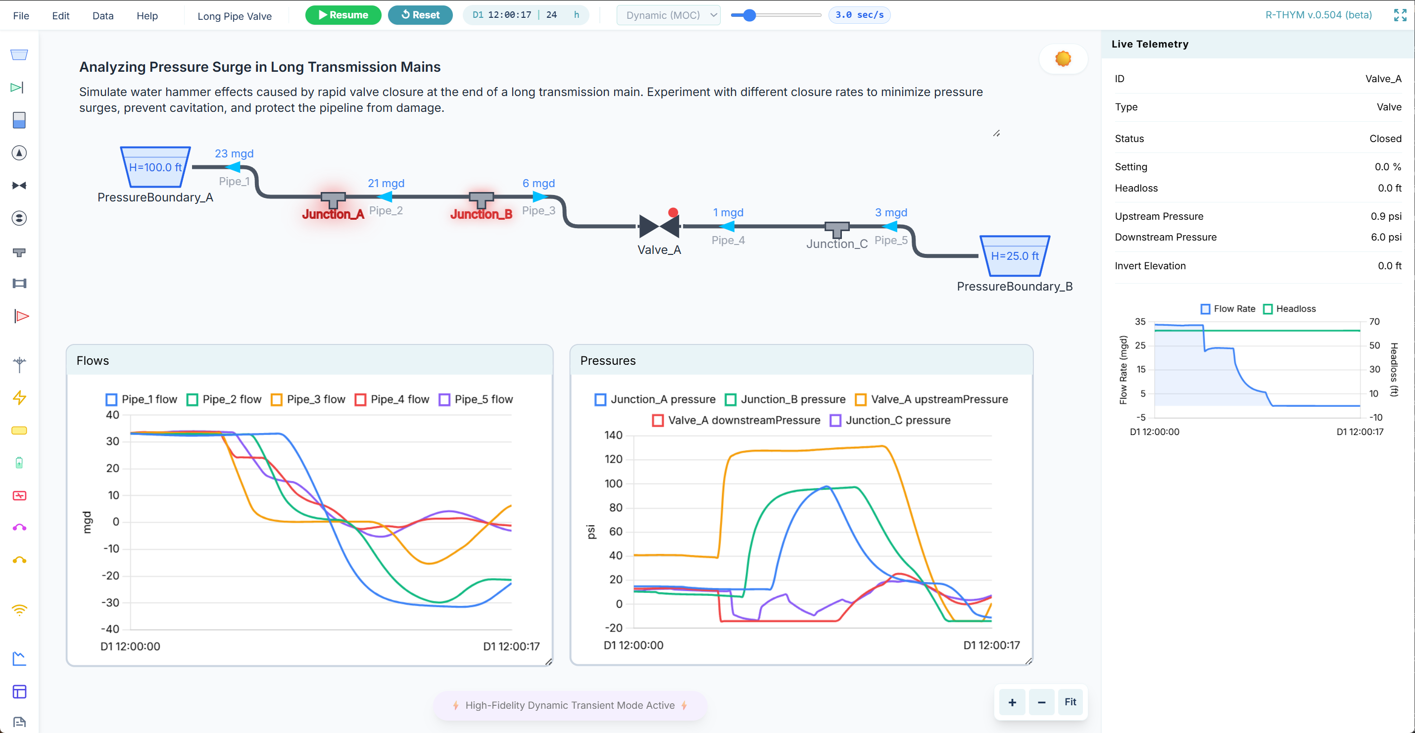
The model represents a municipal bulk transmission line feeding a downstream storage reservoir:
- Upstream Reservoir (PressureBoundary_A): Constant head $H = 100.0\text{ ft}$ ($43.3\text{ psi}$).
- Transmission Main (Pipe_1, Pipe_2, Pipe_3): 3,000 ft of 36-inch HDPE pipe (DR 17, wall thickness 2.12 in, roughness $C = 150$).
- Intermediate Terrain: Junction_A at elevation $66.0\text{ ft}$ ($Station\ 10+00$) and Junction_B at elevation $76.0\text{ ft}$ ($Station\ 20+00$).
- Control Valve (Valve_B): 8-inch high-performance Throttle Control Valve (TCV) located at $Station\ 30+00$ (elevation $0.0\text{ ft}$).
- Downstream Section (Pipe_4, Pipe_5): 1,000 ft of 36-inch pipe discharging into PressureBoundary_B at head $H = 25.0\text{ ft}$ ($10.8\text{ psi}$).
- Transient Event: Valve_B undergoes a rapid 1.0-second linear emergency closure from initial operating setting to $0\%$ open.
Physical Properties & Acoustic Speed
Using the elastic water hammer relation with pipe wall elasticity:
$$a = \sqrt{\frac{K / \rho}{1 + \left(\frac{K}{E}\right)\left(\frac{D}{e}\right) c_1}}$$For 36" HDPE ($E = 110,000\text{ psi}$), R-THYM computes an acoustic celerity:
$$a = 746.7\text{ ft/s}$$The pipe acoustic round-trip reflection time ($2L/a$) upstream of the valve is:
$$T_r = \frac{2 \cdot L}{a} = \frac{2 \cdot 3,000\text{ ft}}{746.7\text{ ft/s}} \approx 8.03\text{ seconds}$$Because valve closure time ($t_c = 1.0\text{ s}$) is significantly less than the critical reflection time ($t_c < 2L/a$), this event qualifies as rapid closure, generating the maximum theoretical Joukowsky surge.
Example Chart 1: Flow Deceleration & Wave Stepping
By setting up a History Chart tracking flow rate (gpm) across Pipe_1, Pipe_2, Pipe_3, Pipe_4, and Pipe_5, we observe the acoustic deceleration waves reflecting through the main.
Pipeline Flow vs. Time During Valve Closure
Key Takeaways from the Flow Chart:
- Steady State ($t < 22.6\text{ s}$): All five pipe segments maintain a constant steady discharge of $Q_0 \approx 544.8\text{ gpm}$.
- Valve Throttling ($22.6\text{ s} \le t \le 32.8\text{ s}$): Flow in Pipe_3 (directly upstream of the valve) decelerates rapidly to zero as the disc seats.
- Wave Propagation Lag: Notice how flow in Pipe_1 (at the reservoir 3,000 ft upstream) remains completely unaffected for approximately $4.0\text{ seconds}$ after valve movement begins ($\Delta t = L/a = 3000 / 746.7 \approx 4.01\text{ s}$). The upstream fluid cannot react until the acoustic compression wave arrives.
Example Chart 2: Pressure Surge Waveforms
Next, we inspect the transient pressure waveforms on a History Chart configured with:
- Y1 Axis: Pressures (psi) at Junction_A, Junction_B, Valve_B (upstream), and Valve_B (downstream).
Acoustic Pressure Oscillations (Water Hammer Waveforms)
Simulation Peak Verification Data:
| Location | Elevation | Steady Pressure | Min Transient | Max Transient | Time of Peak ($t_{max}$) |
|---|---|---|---|---|---|
PressureBoundary_A |
$0.0\text{ ft}$ | $43.29\text{ psi}$ ($100.0\text{ ft}$) | $43.29\text{ psi}$ | $43.29\text{ psi}$ | Fixed Boundary |
Junction_A |
$66.0\text{ ft}$ | $14.73\text{ psi}$ ($100.0\text{ ft}$) | $12.01\text{ psi}$ | $17.87\text{ psi}$ | $t = 36.97\text{ s}$ |
Junction_B |
$76.0\text{ ft}$ | $10.40\text{ psi}$ ($100.0\text{ ft}$) | $6.05\text{ psi}$ | $14.99\text{ psi}$ | $t = 38.39\text{ s}$ |
Valve_B (Upstream) |
$0.0\text{ ft}$ | $43.28\text{ psi}$ ($100.0\text{ ft}$) | $38.39\text{ psi}$ | $48.21\text{ psi}$ | $t = 39.61\text{ s}$ |
Valve_B (Downstream) |
$0.0\text{ ft}$ | $10.84\text{ psi}$ ($25.0\text{ ft}$) | $8.26\text{ psi}$ | $12.80\text{ psi}$ | Downstream Relief |
Analysis of the Waveforms:
1. Upstream Compression Surge: Rapid valve closure converts kinetic flow energy into acoustic pressure head. Upstream pressure jumps from $43.28\text{ psi}$ to $48.21\text{ psi}$ at $t = 39.61\text{ s}$.
2. Intermediate Peak Sequence: The peak occurs progressively earlier moving upstream: $t = 39.61\text{ s}$ at the valve face, $t = 38.39\text{ s}$ at Junction_B, and $t = 36.97\text{ s}$ at Junction_A, matching the physical propagation speed $\Delta t = \Delta x / a$.
3. Downstream Depressurization: Downstream of Valve_B, flow cutoff initiates a negative expansion wave, causing pressure to drop abruptly before stabilizing at downstream boundary head.
Example Chart 3: Longitudinal HGL Profile & Envelopes
The most powerful diagnostic for pipeline integrity is the Longitudinal Profile Chart, which plots the spatial envelope along the full $4,000\text{ ft}$ corridor.
Longitudinal Hydraulic Grade Line (HGL) Profile & Transient Envelopes
Crucial Engineering Insights from the Profile:
- Surge Gradient ($H_{max}$): The maximum transient head increases linearly from the fixed reservoir boundary ($100.0\text{ ft}$) up to $111.3\text{ ft}$ at the valve face. The pipeline structural design must ensure that the pressure class of the 36" HDPE pipe exceeds this maximum pressure everywhere along the corridor.
- High-Point Cavitation Risk ($H_{min}$): Note the hill at $Station\ 20+00$ (Junction_B), where pipe elevation rises to $76.0\text{ ft}$. While steady-state head provides a comfortable $10.4\text{ psi}$, the negative wave swing depresses the minimum transient head to $89.9\text{ ft}$, leaving only $6.05\text{ psi}$ of positive head. If the valve closed even faster (e.g., $0.5\text{ s}$), the $H_{min}$ curve would drop below the pipe invert, creating sub-atmospheric column separation and severe water hammer risks.
Interacting with and Exporting Chart Data
Interactive Crosshair & Tooltips
Hovering your mouse over any active chart displays a synchronized cursor tracking the exact value, timestamp, and component name for all active series.
Pan & Zoom Controls
- Zoom In/Out: Use the mouse scroll wheel over the plot canvas, or click and drag a rectangular zoom window.
- Reset Zoom: Double-click anywhere on the chart plot area to restore the default full scale.
- Pan: Hold
Shiftwhile dragging to pan horizontally through historical timesteps.
Exporting Traces
- Direct CSV Export: In the upper right corner of any chart container, click the Export (⬇) icon to download the active series data as a clean, spreadsheet-ready
.csvfile. - High-Resolution Image: Click the Camera (📷) icon to save an executive presentation image (
.png) of the current chart view. - Complete Simulation Archive: For comprehensive documentation, select Data → MOC Verification Report from the main menu bar to download a
.ziparchive containing the full high-resolution mathematical matrices across every pipe node and calculation grid section.